Large language model inference

LLM inference

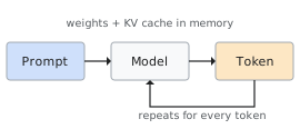
The autoregressive loop: every generated token is fed back as input.

Definition	Using an already trained model to generate text
Basic unit	Token (≈ ¾ of a word in English)
Phases	Prefill, decode
Bottleneck	Memory bandwidth (in the decode phase)
Key techniques	KV cache, batching, quantization
Metrics	TTFT, TPOT, throughput
Typical software	vLLM, TensorRT-LLM, llama.cpp, Hugging Face TGI
Hardware	GPUs, TPUs, dedicated accelerators

Large language model inference (LLM inference) is the process by which an already trained model receives an input text, called the prompt, and produces an output text. It is distinct from training, the phase in which the model learns its parameters: during inference the parameters stay fixed and are only used.

Inference accounts for most of the running cost of an LLM in production, because a model is trained once but queried millions of times. Optimizing it has therefore become an engineering field in its own right, concerned with reducing latency, increasing the number of requests served and keeping memory usage under control. The main techniques are the KV cache, batching and quantization.

Autoregressive generation

Modern LLMs, based on the Transformer architecture,¹ generate text autoregressively: they produce one token at a time, and each new token depends on all the tokens before it. The procedure is:

1. the model receives the available token sequence (the prompt plus everything generated so far);
2. for each token in the vocabulary it computes a score called a logit, which is turned into a probability;
3. it picks the next token based on these probabilities;
4. it appends the chosen token to the sequence and starts again from step 1.

The loop stops when the model produces a special end-of-sequence token or when the maximum number of tokens is reached.

Tokens and tokenization

A token is the smallest unit of text the model works with. It is not the same as a word: it can be a whole word, part of a word or a punctuation mark. Splitting text into tokens is called tokenization and usually relies on algorithms such as Byte Pair Encoding (BPE). In English a token corresponds on average to about three quarters of a word; languages that are less represented in the training data, such as Italian, often need more tokens for the same sentence.

Choosing the next token

The rule used to pick the token is called the decoding strategy or sampling strategy:

• Greedy: always take the most likely token. It is deterministic but tends to produce repetitive text.
• Temperature: a parameter that makes the distribution “flatter” (high values, more varied text) or “sharper” (low values, more predictable text).
• Top-k: sample only among the k most likely tokens.
• Top-p (or nucleus sampling): sample among the most likely tokens whose cumulative probability reaches the threshold p.

Phases of inference

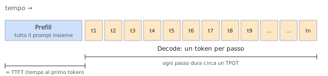
Figure 1. Timeline of a request: a single prefill step, then many decode steps, one for each generated token.

Serving a single request happens in two phases with very different characteristics. Many optimizations only make sense once this distinction is clear.

Prefill

In the prefill phase (also called prompt processing) the model reads the whole prompt in a single pass. Since all the prompt tokens are already known, they can be processed in parallel with large matrix multiplications. This phase is therefore compute-bound and uses the hardware well. At the end of prefill the model produces the first token of the answer and fills the KV cache with the prompt’s data.

Decode

In the decode phase (or generation) the model generates the following tokens one at a time, because each one depends on the previous one. At every step it processes a single new token, but it still has to read all the model weights and the KV cache from memory. There is little computation compared with the amount of data to move, so this phase is memory-bound (see below). Decode usually takes most of the total time of a request.

Comparison of the two phases

Property	Prefill	Decode
Tokens processed per step	All the prompt tokens	One
Parallelism	High	Low (sequential)
Limiting resource	Compute	Memory bandwidth
Related metric	TTFT	TPOT

Memory

Accelerator memory (for example a GPU’s VRAM) is the scarcest resource during inference. It is taken up mainly by two things: the model weights and the KV cache.

Model weights

The weights are the parameters learned during training. The memory they take up follows a simple formula:

$\text{weight memory}=\text{number of parameters}\times \text{bytes per parameter}$

The number of bytes depends on the numeric format used (see Quantization).

Memory taken up by the weights alone of a 7-billion-parameter model

Format	Bytes per parameter	Memory
FP32	4	≈ 28 GB
FP16 / BF16	2	≈ 14 GB
INT8	1	≈ 7 GB
INT4	0.5	≈ 3.5 GB

KV cache

In the Transformer’s attention mechanism, every token produces two vectors called the key (K) and the value (V), which later tokens use to “look at” the past. Without any precaution, at every decode step the model would have to recompute K and V for all previous tokens, repeating work it has already done.

The KV cache avoids this waste: it stores K and V for every token already processed, so each step only computes them for the new token. It is a classic memory–compute trade-off: more memory is used in exchange for far less computation.

Its size grows linearly with the length of the text and with the number of requests served together:

$\text{KV cache}=2\times \text{layers}\times \text{model dim.}\times \text{bytes per value}\times \text{tokens}\times \text{requests}$

(the 2 counts both K and V)

Example. For a model with 32 layers and dimension 4096 in FP16 (2 bytes), such as Llama 2 7B, each token takes 2 × 32 × 4096 × 2 = 524,288 bytes, i.e. about 0.5 MB. A 4096-token conversation needs about 2 GB of KV cache; 8 conversations of that length served together need about 16 GB, more than the weights themselves.

This is why the KV cache is often what limits how many requests can be served at the same time. Some solutions:

• PagedAttention, introduced with the vLLM system: it manages the KV cache in fixed-size blocks, like an operating system’s virtual memory, reducing the waste caused by fragmentation.²
• Grouped-Query Attention (GQA) and Multi-Query Attention (MQA): architectural variants in which several attention “heads” share the same K and V, shrinking the cache.³
• KV cache quantization: K and V are stored with fewer bits.

The memory bandwidth limit

This is the most important idea in this entry: it explains why almost all the other techniques exist.

An accelerator has two separate capacities: how many operations it can perform per second (compute, measured in FLOPS) and how much data it can read from memory per second (memory bandwidth, measured in GB/s). An operation is compute-bound if it is limited by the former, memory-bound if it is limited by the latter.

The ratio between operations performed and bytes read is called arithmetic intensity. In decode with a single request, about 2 operations are performed for every parameter read (2 bytes in FP16): the intensity is about 1 operation per byte. Modern GPUs, on the other hand, need hundreds of operations per byte to be fully used. The result is that, during decode, the compute units spend most of their time waiting for data.

This gives an upper bound on the generation speed of a single request:

$\text{tokens per second (max)}\approx \frac{\text{memory bandwidth}}{\text{model size in bytes}}$

Example. A 14 GB model (7B in FP16) on an accelerator with 1,000 GB/s of bandwidth cannot exceed about 1,000 ÷ 14 ≈ 70 tokens per second for a single request, whatever its compute power.

Optimization techniques attack this limit in two ways:

• reading fewer bytes: the purpose of quantization;
• doing more work per read: the purpose of batching, because weights read once serve several requests.

Batching

Batching means processing several requests together in a single pass of the model. Since in decode the main cost is reading the weights, serving 16 requests together costs little more than serving one: the weights are read once and used for all of them. Overall throughput, i.e. the tokens generated per second summed over all users, therefore increases a lot.

There are several forms of batching:

• Static batching: a group of requests is collected and processed until all of them have finished. It is simple, but one long answer makes the others, already finished, wait, and the freed slots stay unused.
• Dynamic batching: the group is formed from the requests that arrive within a short time window. It reduces the wait to form the group, but once started it has the same limits as static batching.
• Continuous batching (or in-flight batching, iteration-level scheduling): the composition of the group is updated at every decode step. As soon as a request finishes, its slot is taken by a new one. The hardware stays busy all the time. It is the technique used by the main modern serving systems.⁴

Latency–throughput trade-off. Larger batches increase total throughput but make each step a little slower, so each individual user receives tokens slightly later. In addition, every extra request takes space in the KV cache. The batch size is chosen by balancing these three factors.

Quantization

Quantization is the representation of the weights (and sometimes of activations and the KV cache) with reduced-precision numbers, i.e. with fewer bits. Models are usually trained in FP32 or BF16 and then converted, for inference, to formats such as INT8 or INT4.

There are two advantages: the model takes up less memory (it fits on smaller hardware, or leaves more room for the KV cache) and, since decode is memory-bound, it generates faster, because it reads fewer bytes at every step. The drawback is a loss of accuracy, usually small at 8 bits and more noticeable at 4 bits or below.

Common numeric formats

Format	Bits	Type	Typical use
FP32	32	Floating point	Training (historically)
BF16	16	Floating point	Training and inference
FP16	16	Floating point	Inference
FP8	8	Floating point	Inference on recent hardware
INT8	8	Integer	Inference
INT4	4	Integer	Inference on limited hardware

Classification

• By when it happens:
  • Post-Training Quantization (PTQ): an already trained model is quantized. It is the most common form because it does not require retraining.
  • Quantization-Aware Training (QAT): the model is trained “knowing” it will be quantized, so it loses less quality.
• By what is quantized:
  • Weights only (weight-only): memory is reduced, but the computations still run at high precision.
  • Weights and activations: the computations also run at low precision, if the hardware supports it.

Well-known methods include LLM.int8(),⁵ GPTQ⁶ and AWQ.⁷

Performance metrics

The performance of an inference system is measured with a few standard metrics:

Abbreviation	Name	Meaning	Depends mainly on
TTFT	Time To First Token	Time between sending the request and receiving the first token	Prefill, queueing
TPOT / ITL	Time Per Output Token / Inter-Token Latency	Average time between one token and the next	Decode, batch size
Latency	End-to-end latency	Total time to get the complete answer	Both phases
Throughput	Throughput	Tokens (or requests) produced per second by the whole system	Batching, hardware

The total latency of an answer of n tokens can be approximated as:

$\text{latency}\approx \text{TTFT}+\text{TPOT}\times (n-1)$

TTFT matters most in interactive applications such as chat, because it is the moment the user sees the answer “start”. Throughput matters most for costs: more tokens per second means serving more users with the same hardware. When comparing two configurations, tail values such as the 95th or 99th percentile (p95, p99) are usually considered as well, not just the average.

Other optimization techniques

• FlashAttention: an implementation of attention that reorganizes the computation to reduce reads and writes to main memory, making it faster without changing the result.⁸
• Speculative decoding: a small, fast model “guesses” several tokens ahead, and the large model verifies them all together in a single step. If the guesses are right, more tokens are generated per step.⁹
• Parallelism: when a model does not fit on a single accelerator, it is split across several devices. In tensor parallelism each layer is split across the devices; in pipeline parallelism each device runs a group of layers.
• Prefix caching: if many requests start with the same text (for example the same system prompt), the KV cache of that shared part is computed once and reused.
• Chunked prefill: very long prompts are split into chunks and interleaved with the decode steps of other requests, so that one long prompt does not block all the other users.

Hardware

LLM inference usually runs on accelerators, i.e. processors specialized in parallel matrix computations. The properties that matter most are the amount of memory (how large the model plus the KV cache can be), memory bandwidth (how fast decode is) and support for low-precision formats (how much is gained from quantization).

• GPUs: the most widespread accelerators, especially NVIDIA’s, used with software such as vLLM and TensorRT-LLM.
• TPUs: accelerators designed by Google for machine learning.
• Dedicated accelerators: chips designed by other companies for inference. Among them is IBM Spyre, a PCIe card designed to run AI models, including LLMs, on IBM Z mainframes and LinuxONE systems, close to companies’ data.¹⁰ The same principles described in this entry apply to these devices: memory management, batching, quantization and performance measurement.

English–Italian glossary

Terms commonly used in English even in Italian contexts, with an example sentence useful in a job interview.

Term	Italian	Example sentence
Inference	Inferenza: uso del modello addestrato	Inference is when we use a trained model to generate output.
Autoregressive	Autoregressivo: un token alla volta	An LLM generates text one token at a time.
Prefill / decode	Lettura del prompt / generazione della risposta	Prefill reads the prompt in parallel; decode generates tokens one by one.
KV cache	Memoria di K e V dei token passati	The KV cache stores past keys and values, so we don’t recompute them.
Memory-bound	Limitato dalla banda di memoria	Decode is memory-bound: for each token we read all the weights.
Batching	Elaborare più richieste insieme	Batching uses the weights for many requests at once.
Continuous batching	Il batch cambia a ogni passo	New requests join as soon as others finish.
Quantization	Quantizzazione: numeri con meno bit	Quantization makes the model smaller and faster, with a small loss in quality.
TTFT	Tempo al primo token	TTFT is how long the user waits before the answer starts.
Throughput	Token al secondo dell’intero sistema	Bigger batches give higher throughput but higher latency per user.
Profiling	Misurare dove si spende il tempo	I profile the system to find where time is spent.

See also

• Transformer architecture
• Attention mechanism
• Retrieval-augmented generation
• Graphics processing unit
• Roofline model
• Virtual memory
• Neural network training
• Knowledge distillation

References

Footnotes

1. Vaswani, A. et al. (2017). Attention Is All You Need. NeurIPS. arXiv:1706.03762 ↩

2. Kwon, W. et al. (2023). Efficient Memory Management for Large Language Model Serving with PagedAttention. SOSP. arXiv:2309.06180 ↩

3. Ainslie, J. et al. (2023). GQA: Training Generalized Multi-Query Transformer Models from Multi-Head Checkpoints. EMNLP. arXiv:2305.13245 ↩

4. Yu, G.-I. et al. (2022). Orca: A Distributed Serving System for Transformer-Based Generative Models. OSDI. usenix.org ↩

5. Dettmers, T. et al. (2022). LLM.int8(): 8-bit Matrix Multiplication for Transformers at Scale. NeurIPS. arXiv:2208.07339 ↩

6. Frantar, E. et al. (2022). GPTQ: Accurate Post-Training Quantization for Generative Pre-trained Transformers. ICLR 2023. arXiv:2210.17323 ↩

7. Lin, J. et al. (2023). AWQ: Activation-aware Weight Quantization for LLM Compression and Acceleration. MLSys 2024. arXiv:2306.00978 ↩

8. Dao, T. et al. (2022). FlashAttention: Fast and Memory-Efficient Exact Attention with IO-Awareness. NeurIPS. arXiv:2205.14135 ↩

9. Leviathan, Y., Kalman, M., Matias, Y. (2023). Fast Inference from Transformers via Speculative Decoding. ICML. arXiv:2211.17192 ↩

10. IBM. Product pages for the IBM Spyre Accelerator and IBM z17. Technical specifications should be checked against the official IBM documentation: ibm.com ↩